正则化是在损失函数中给每个参数 w 加上权重,引入模型复杂度指标,从而抑制模型噪声,减小过拟合。
过拟合:
神经网络模型在训练数据集上的准确率较高,在新的数据进行预测或分类时准确率较 低,说明模型的泛化能力差。
使用正则化后,损失函数 loss 变为两项之和:
loss = loss(y 与 y_) + REGULARIZER*loss(w) 其中,第一项是预测结果与标准答案之间的差距,如之前讲过的交叉熵、均方误差等;第二项是正则
化计算结果。
正则化计算方法:
1 L1 正则化: 𝒍𝒐𝒔𝒔𝑳𝟏 = ∑𝒊|𝒘𝒊|
用 Tesnsorflow 函数表示:loss(w) = tf.contrib.layers.l1_regularizer(REGULARIZER)(w) 2 L2 正则化: 𝒍𝒐𝒔𝒔𝑳𝟐 = ∑𝒊|𝒘𝒊|𝟐
用 Tesnsorflow 函数表示:loss(w) = tf.contrib.layers.l2_regularizer(REGULARIZER)(w) √用 Tesnsorflow 函数实现正则化:
tf.add_to_collection(‘losses’, tf.contrib.layers.l2_regularizer(regularizer)(w) loss = cem + tf.add_n(tf.get_collection(‘losses’))
cem 的计算已在 4.1 节中给出。
举例:
在本例子中,使用了之前未用过的模块与函数:
matplotlib 模块:
Python 中的可视化工具模块,实现函数可视化终端安装指令:sudo pip install matplotlib
函数 plt.scatter():
利用指定颜色实现点(x,y)的可视化 plt.scatter (x 坐标, y 坐标, c=”颜色”)
plt.show()
收集规定区域内所有的网格坐标点:
xx, yy = np.mgrid[起:止:步长, 起:止:步长] #找到规定区域以步长为分辨率的行列网格坐标点 grid = np.c_[xx.ravel(), yy.ravel()] #收集规定区域内所有的网格坐标点 √plt.contour()函数:告知 x、y 坐标和各点高度,用 levels 指定高度的点描上颜色 plt.contour (x 轴坐标值, y 轴坐标值, 该点的高度, levels=[等高线的高度])
plt.show()
代码如下:1
2
3
4
5
6
7
8
9
10
11
12
13
14
15
16
17
18
19
20
21
22
23
24
25
26
27
28
29
30
31
32
33
34
35
36
37
38
39
40
41
42
43
44
45
46
47
48
49
50
51
52
53
54
55
56
57
58
59
60
61
62
63
64
65
66
67
68
69
70
71
72
73
74
75
76
77
78
79
80
81
82
83
84
85
86
87
88
89
90
91
92
93
94
95
96
97
98
99
100
101
102
103
104
105
106
107
108
109#coding:utf-8
#0导入模块 ,生成模拟数据集
import tensorflow as tf
import numpy as np
import matplotlib.pyplot as plt
BATCH_SIZE = 30
seed = 2
#基于seed产生随机数
rdm = np.random.RandomState(seed)
#随机数返回300行2列的矩阵,表示300组坐标点(x0,x1)作为输入数据集
X = rdm.randn(300,2)
#从X这个300行2列的矩阵中取出一行,判断如果两个坐标的平方和小于2,给Y赋值1,其余赋值0
#作为输入数据集的标签(正确答案)
Y_ = [int(x0*x0 + x1*x1 <2) for (x0,x1) in X]
#遍历Y中的每个元素,1赋值'red'其余赋值'blue',这样可视化显示时人可以直观区分
Y_c = [['red' if y else 'blue'] for y in Y_]
#对数据集X和标签Y进行shape整理,第一个元素为-1表示,随第二个参数计算得到,第二个元素表示多少列,把X整理为n行2列,把Y整理为n行1列
X = np.vstack(X).reshape(-1,2)
Y_ = np.vstack(Y_).reshape(-1,1)
print X
print Y_
print Y_c
#用plt.scatter画出数据集X各行中第0列元素和第1列元素的点即各行的(x0,x1),用各行Y_c对应的值表示颜色(c是color的缩写)
plt.scatter(X[:,0], X[:,1], c=np.squeeze(Y_c))
plt.show()
#定义神经网络的输入、参数和输出,定义前向传播过程
def get_weight(shape, regularizer):
w = tf.Variable(tf.random_normal(shape), dtype=tf.float32)
tf.add_to_collection('losses', tf.contrib.layers.l2_regularizer(regularizer)(w))
return w
def get_bias(shape):
b = tf.Variable(tf.constant(0.01, shape=shape))
return b
x = tf.placeholder(tf.float32, shape=(None, 2))
y_ = tf.placeholder(tf.float32, shape=(None, 1))
w1 = get_weight([2,11], 0.01)
b1 = get_bias([11])
y1 = tf.nn.relu(tf.matmul(x, w1)+b1)
w2 = get_weight([11,1], 0.01)
b2 = get_bias([1])
y = tf.matmul(y1, w2)+b2
#定义损失函数
loss_mse = tf.reduce_mean(tf.square(y-y_))
loss_total = loss_mse + tf.add_n(tf.get_collection('losses'))
#定义反向传播方法:不含正则化
train_step = tf.train.AdamOptimizer(0.0001).minimize(loss_mse)
with tf.Session() as sess:
init_op = tf.global_variables_initializer()
sess.run(init_op)
STEPS = 40000
for i in range(STEPS):
start = (i*BATCH_SIZE) % 300
end = start + BATCH_SIZE
sess.run(train_step, feed_dict={x:X[start:end], y_:Y_[start:end]})
if i % 2000 == 0:
loss_mse_v = sess.run(loss_mse, feed_dict={x:X, y_:Y_})
print("After %d steps, loss is: %f" %(i, loss_mse_v))
#xx在-3到3之间以步长为0.01,yy在-3到3之间以步长0.01,生成二维网格坐标点
xx, yy = np.mgrid[-3:3:.01, -3:3:.01]
#将xx , yy拉直,并合并成一个2列的矩阵,得到一个网格坐标点的集合
grid = np.c_[xx.ravel(), yy.ravel()]
#将网格坐标点喂入神经网络 ,probs为输出
probs = sess.run(y, feed_dict={x:grid})
#probs的shape调整成xx的样子
probs = probs.reshape(xx.shape)
print "w1:\n",sess.run(w1)
print "b1:\n",sess.run(b1)
print "w2:\n",sess.run(w2)
print "b2:\n",sess.run(b2)
plt.scatter(X[:,0], X[:,1], c=np.squeeze(Y_c))
plt.contour(xx, yy, probs, levels=[.5])
plt.show()
#定义反向传播方法:包含正则化
train_step = tf.train.AdamOptimizer(0.0001).minimize(loss_total)
with tf.Session() as sess:
init_op = tf.global_variables_initializer()
sess.run(init_op)
STEPS = 40000
for i in range(STEPS):
start = (i*BATCH_SIZE) % 300
end = start + BATCH_SIZE
sess.run(train_step, feed_dict={x: X[start:end], y_:Y_[start:end]})
if i % 2000 == 0:
loss_v = sess.run(loss_total, feed_dict={x:X,y_:Y_})
print("After %d steps, loss is: %f" %(i, loss_v))
xx, yy = np.mgrid[-3:3:.01, -3:3:.01]
grid = np.c_[xx.ravel(), yy.ravel()]
probs = sess.run(y, feed_dict={x:grid})
probs = probs.reshape(xx.shape)
print "w1:\n",sess.run(w1)
print "b1:\n",sess.run(b1)
print "w2:\n",sess.run(w2)
print "b2:\n",sess.run(b2)
plt.scatter(X[:,0], X[:,1], c=np.squeeze(Y_c))
plt.contour(xx, yy, probs, levels=[.5])
plt.show()
执行代码,效果如下:
首先,数据集实现可视化,x0 + x1 < 2 的点显示红色, x0 + x1 ≥2 的点显示蓝色,如图所示: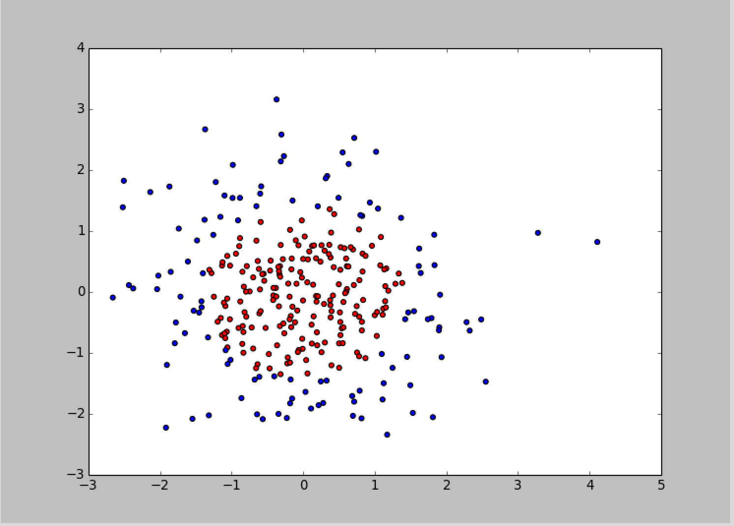
接着,执行无正则化的训练过程,把红色的点和蓝色的点分开,生成曲线如下图所示: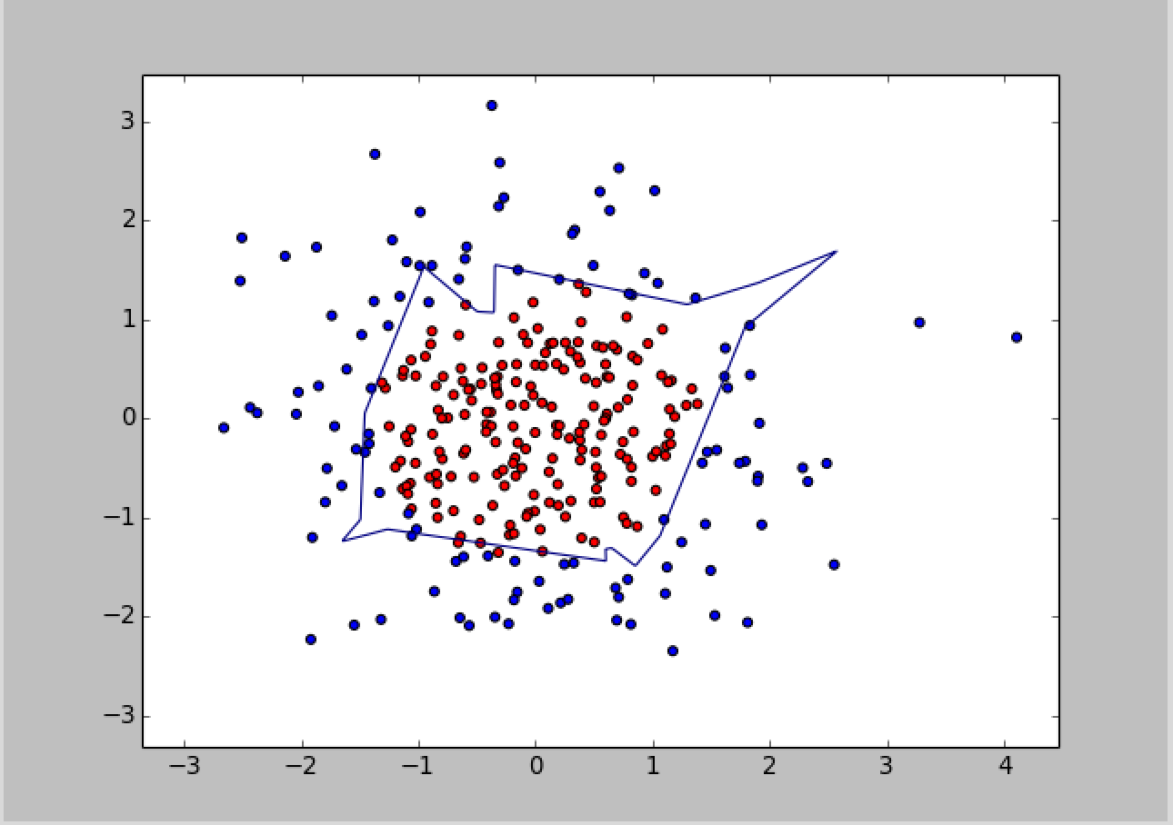
最后,执行有正则化的训练过程,把红色的点和蓝色的点分开,生成曲线如下图所示: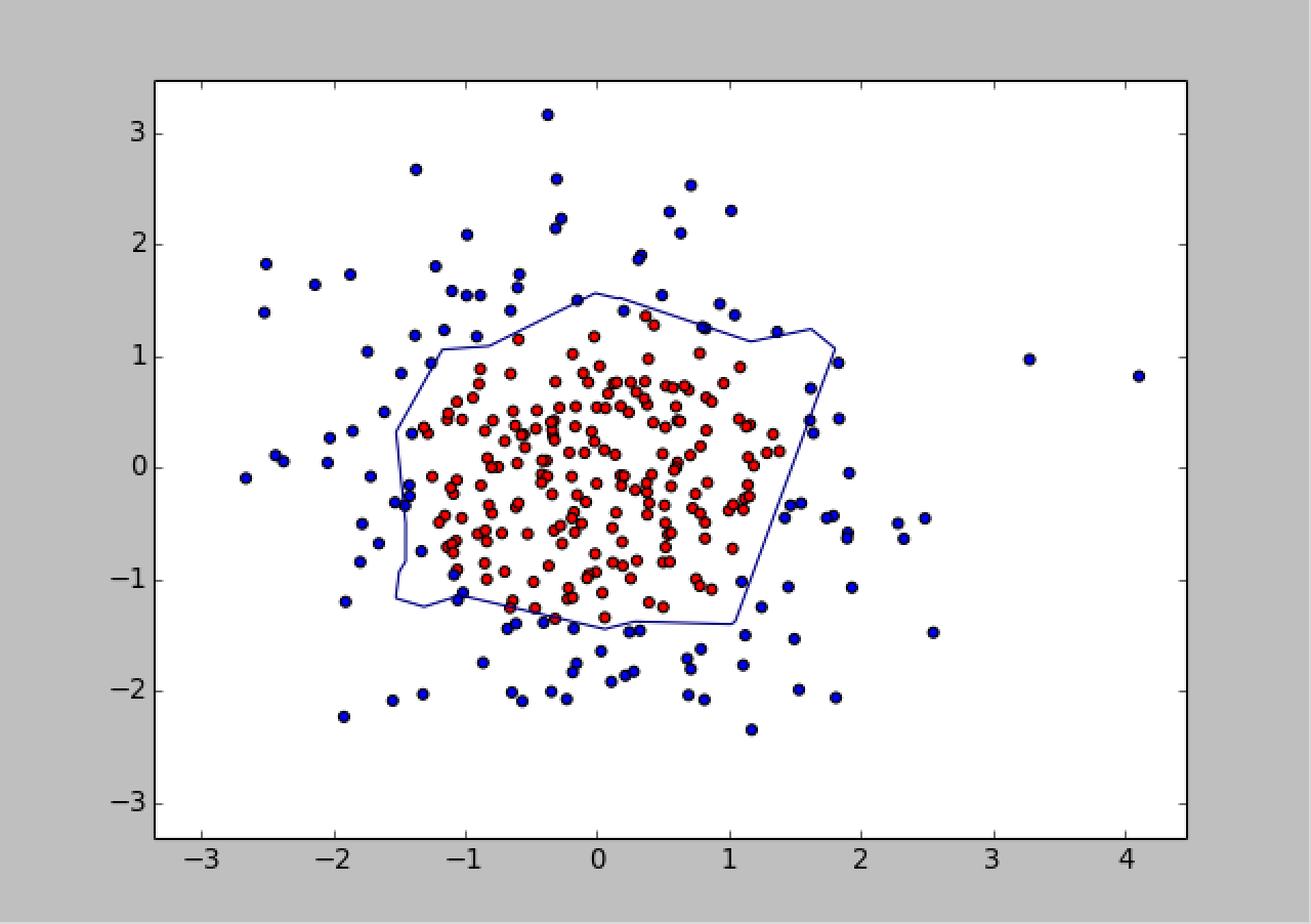
对比无正则化与有正则化模型的训练结果,可看出有正则化模型的拟合曲线平滑,模型具有更好的泛化能力。
代码实现参考Githubopt_regular.py